To nest, or not to nest? Nested data types in Polars with big data

It was a pleasure to give a talk at this year’s PyData conference, my first time presenting at the event. It was well-organised, with top-quality talks, and a great vibe amongst attendees. This post is follow-on from my talk about nested data types in the Polars dataframe library. It goes a little further than the presentation, since there were many relevant questions and remarks in the Q&A session afterwards.

My talk was inspired by a data pipeline I was working on last summer. I had collected snapshots of crypto order book data, as part of my research, and was importing data from centralised exchanges into Polars. Order book data is typically stored in JSON format, with a nested structure, and I went down a bit of rabbit hole exploring the different options for representing this within Polars. This rabbit hole developed into a wider exploration of the storage and performance implications of nested types, as well as the impact on query structure, with a set of reproducible benchmarks.

The start of the presentation included a basic introduction to Polars nested types, which I won’t touch upon in this blog post. But the slides are available here, and the full repository is online here - I make reference to this throughout this post. The following is intended to describe the data I’ve used for the benchmarking, the queries I’ve tested, the results of the benchmarks, and what that means for users of Polars. If you need a reminder of nested types, I refer you to the documentation on lists and arrays.

A few caveats:

• The title of my talk says “big data”, however, I’m only really testing Polars’ in-memory capability here, not the streaming functionality.
• I’m focused on use in Python, not in Polars’ native Rust, or other bindings such as NodeJS or R.
• This is about practical use, not the technical details of how Polars implements nested types.
• There isn’t any benchmarking against other columnar databases such as DuckDB or distributed approaches like Spark.
• If you’re not interested in financial data, skip to the benchmarking.

Data simulation

Central limit order books are the predominant economic design for matching buyers and sellers on trading venues. For crypto exchanges, the JSON structure for a snapshot of an order book typically looks like this:

{
    "lastUpdateId": 55069433,
    "bids": [
        [
            "1.00080000",
            "31856.30000000"
        ],
        [
            ...
        ]
    ],
    "asks": [
        [
            "1.00090000",
            "25718.40000000"
        ],
        [
            ...
        ]
    ]
}

Each side of the book, bids and asks, is represented by an array with a length corresponding to the number of price levels, and an inner array with 2 elements - the price and quantity. Additionally, there is a field providing an ID. The above example was collected from Binance in real time, so there is also a corresponding timestamp for when the snapshot was collected. The structure of this data potentially makes it ideal for storing in a nested type, but it can also be used for testing whether this is optimal.

In order to make a set of reproducible benchmarks, I simulate an order book over time using NumPy, demonstrating a real-world example. In the repo, the simulation is carried out in lob_data.py. Firstly, a random walk represents the price evolving over time:

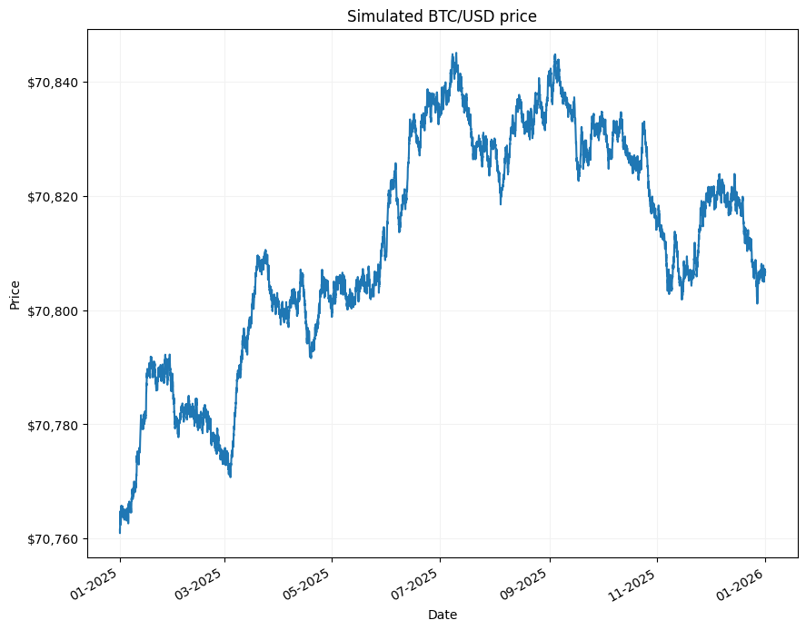
These simulated prices cover the whole of 2025, with an observation each hour. Then from these prices I construct an imaginary order book using the function create_book(). This function uses a power distribution to shape each side of the book, and randomly scales the total volume on each side, as well as the spread (the difference between the highest bid and lowest ask). This is designed to somewhat mimic a real-life order book, and means that little to none of the data points are repeated.

Graphing the simulated data for $t = 0, 1, 2, 3$ demonstrates how the order book evolves over time:

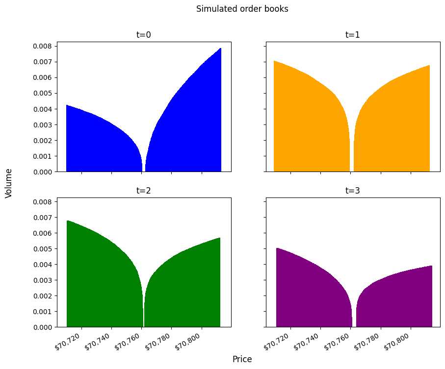
Importantly, we create two versions of these simulated order books, with a fixed number of levels and a variable number of levels. This is significant later on, when we test both Polars’ arrays and lists, which are intended for fixed and variable length. For the fixed simulation, each side of the book has 5,000 price levels, and for the variable version each side is randomly trimmed. The simulated data is stored in the pickle format as an intermediary step. These files are approximately 1.4 GB in size, with the variable version slightly smaller.

Specification of nested structure

Given the existing structure of our data, there are several options for representing this in a Polars dataframe. I have opted for what I see as the most logical, covering the main configurations we could choose, for both lists and arrays. Plus, I’ve run these benchmarks for both fixed and variable length order books. Not using any nesting acts as the baseline standard. I have also included the use of structs, which are a composite type, but do enable us to further structure our data in a single column. And, I’ve used both arrays and lists for the fixed length data despite us knowing beforehand that it won’t exceed 5,000 on either side of the book. The intention here is to quantify the difference, especially given that the Polars user guide tells us that arrays are more memory efficient and performant when you’ve got a fixed shape.

Fixed length

i.e. 5,000 levels on the bid and ask side

• No nesting
• Nested array (2 levels of nesting)
• Flat array (1 level of nesting)
• Nested list (2 levels of nesting)
• Flat list (1 level of nesting)
• Struct

Variable length

i.e. Random trimming of bid and ask side $[4900, 4999]$

• No nesting
• Nested list (2 levels of nesting)
• Flat list (1 level of nesting)
• Struct

This is not exhaustive, it might be nice, for instance, to use a struct inside an array. However, I believe these give us a good illustration in terms of performance, etc.

Test environment

The benchmarks are run on a HP laptop with an Intel i5 12th generation CPU, 16GB RAM, SSD, running Ubuntu 24.04.4 LTS and the Linux 6.17.0-23-generic kernel. I’m using Python 3.12.3, Polars 1.39.3, and the timeit library to measure execution time, with 100 repetitions, reporting the minimum value.

JSON and ingest

To make this as close to a real data pipeline as possible, I generate the corresponding JSON files in lob_json.py. The files are named using the timestamp, and on disk are 3.8 GB and 3.7 GB for the fixed and variable versions. So there is no confusion about the nested structures we are imposing on our data, a sample of the corresponding dataframes are in the appendix for reference.

Row counts

Depending on the specification, we have different numbers of rows, according to whether the price levels are exploded into individual row records or nested.

Fixed length

Name	Description	Num. Rows
nonest	No nesting	43,800,000
nestarr	Nested array	8,760
flatarr	Flat array	43,800,000
nestlist	Nested list	8_760
flatlist	Flat list	43,800,000
struct	Struct	43,800,000

Variable length

Name	Description	Num. Rows
nonest	No nesting	43,504,190
nestlist	Nested list	8,760
flatlist	Flat list	43,504,190
struct	Struct	8,760

Results

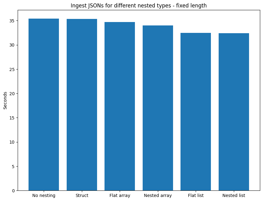
The code for ingesting the JSON files is contained within lob_ingest_fix.py and lob_ingest_var.py, which both make use of pl.scan_ndjson() to lazily read the JSON files. These queries, including the insertion of the timestamp, are appended to a Python list, and combined with pl.concat(), before being collected. The results are as follows:

Fixed length

Structure	Time (secs)
No nesting	35.4
Nested array	34.0
Flat array	34.7
Nested list	32.4
Flat list	32.5
Struct	35.3

The best performing are Nested list and Flat list, speaking to the fact that these types aren’t constrained by a fixed shape. The Nested list is 0.25% faster than the Flat list, demonstrating that there isn’t much penalty to exploding one level of the nested structure, nevertheless, preserving the structure is faster. The arrays come in next, with the Nested array 2.10% quicker than the Flat array, the disadvantage for the fixed shape being slightly higher, in comparison with the list versions. This also once again highlights that preserving the nested structure is more rapid. If we focus on this idea of preserving the structure, the fixed size of the array type makes it 5.00% slower than its list counterpart (comparing Nested array versus Nested list). The last group are the Struct and No nesting. The Struct is marginally quicker than No nesting (0.21% faster), which appears to be due to the difference between splitting up the inner structure into 4 columns (No nesting) compared to retaining the inner structure and dropping the 2 values into a struct. Contrasting the best to the worse performing, Nested list is 8.56% faster than No nesting.

Variable length

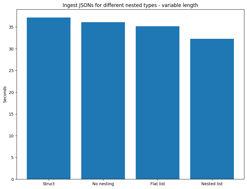
Description	Time (secs)
No nesting	36.1
Nested list	32.3
Flat list	35.1
Struct	37.2

The Nested list is once again the fastest at ingesting the JSON files. And, as for the fixed length data, preserving the nested structure is optimal, with Nested list 8.09% swifter than Flat list. No nesting arrives in third place, being 11.79% slower than duplicating the JSON structure with Nested list. We see a material difference between Struct and No nesting, as opposed to the fixed length data benchmarks. This time, Struct is 2.94% slower than No nesting, which is interesting, since the main difference in the queries is splitting up the inner structures into separate columns or maintaining it in a struct. However, this time the latter approach is penalising. The main issue with all of these structures, bar the Nested list, is the need to pad the shorter side of the book with null values, achieved using a when-then-otherwise expression.

Storage

In this part, I compare the implications of the different nested types on storage. I use the Zstandard compression algorithm, the default in Polars, to write out the parquet files. To account for different levels of compression, I run the full range of levels from 1 to 22.

Fixed length

The sizes in MB are as follows:

Compression	No nesting	Nested array	Flat array	Nested list	Flat list	Struct
1	1034.39	1138.81	1142.71	1138.81	1142.71	1034.39
2	840.12	920.2	936.01	920.2	936.01	840.12
3	829.13	874.86	881.76	874.86	881.76	829.13
4	814.62	872.47	879.35	872.47	879.35	814.62
5	818.91	891.26	897.08	891.26	897.08	818.91
6	818.8	891.24	897.08	891.24	897.08	818.8
7	817.74	892.32	898.18	892.32	898.18	817.74
8	802.0	854.06	861.45	854.06	861.45	802.0
9	801.85	853.8	861.32	853.8	861.32	801.85
10	801.83	853.79	861.31	853.79	861.31	801.83
11	801.82	853.79	861.31	853.79	861.31	801.82
12	801.82	853.79	861.32	853.79	861.32	801.82
13	795.59	843.47	848.61	843.47	848.61	795.59
14	793.22	843.47	848.61	843.47	848.61	793.22
15	793.22	843.47	848.61	843.47	848.61	793.22
16	751.53	828.18	837.85	828.18	837.85	751.53
17	732.41	867.18	876.09	867.18	876.09	732.4
18	679.37	721.01	723.98	721.01	723.98	679.36
19	677.9	719.19	722.63	719.19	722.63	677.91
20	677.9	719.19	722.63	719.19	722.63	677.91
21	677.9	719.13	722.63	719.13	722.63	677.91
22	677.9	718.9	722.63	718.9	722.63	677.91

It is noteworthy that the different structures fall into 3 groups of almost exactly the same size: No nesting and Struct, Nested array and Nested List, Flat array and Flat list. These differ by only a matter of bytes. For example, at compression = 1, Struct is 89 bytes larger than No nesting, Nested array is 16 bytes bigger than Nested list, and Flat array is 4 bytes more voluminous than Flat list. These slight differences are maintained at the other end of the compression scale (22), for Nested array/Nested list and Flat array/Flat list, but not for No nesting/Struct, where the small gap widens slightly.

For the purposes of visual clarity, and to illustrate the broader trends, we chart these 3 groups together.

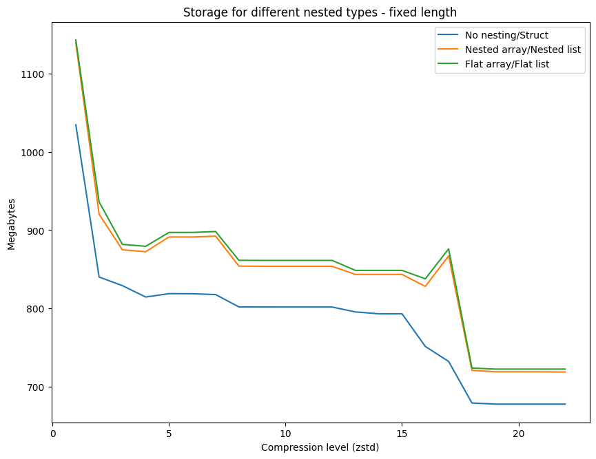
The graph highlights that all data structures see a considerable drop in size between compression level 1 and 2. This is most most pronounced for Nested array/Nested list, which sees a drop in size of more than 218 MB. It is important to point out that Polars defaults to compression level 3 when using Zstandard, which makes sense when we see the considerable reduction in size, although this gain isn’t as prominent between levels 2 and 3. Overall, the overhead for using any of the nested structures is significant and No nesting/Struct are consistently less onerous if hard disk space is at a premium. In addition, there appear to be 3 rough trends for all of the data structures, as we go from level 1 to level 2, then at level 2 onwards the line flattens out, before a further significant drop at the highest levels of compression. The difference between using the nested or flat structures (Nested array versus Flat array, Nested list versus Flat list) is negligible, although the former is marginally smaller. Finally, it is curious that there are a few unusual peaks, where size increases alongside the compression level. This is evident for all data structures around levels 4-6, and for 16-17 for all of the nested structures. For example, with the Flat array size increases by 4.36% from level 16-17.

Variable length

Once again, the sizes in MB are as follows:

Compression	No nesting	Flat list	Struct	Nested list
1	1024.96	1132.12	1024.87	1122.43
2	833.02	927.59	832.7	911.27
3	821.82	874.4	821.1	864.99
4	806.95	871.56	806.27	863.43
5	810.17	888.79	809.62	882.23
6	810.01	888.76	809.46	882.15
7	808.86	889.67	808.36	883.3
8	788.7	852.79	788.32	846.09
9	788.63	852.68	788.23	845.9
10	788.63	852.69	788.21	845.9
11	788.62	852.68	788.21	845.9
12	788.62	852.68	788.21	845.9
13	781.22	840.78	781.41	835.56
14	778.81	840.76	779.0	835.56
15	778.81	840.75	779.0	835.56
16	747.53	827.83	750.16	820.39
17	723.94	867.02	723.19	852.26
18	670.02	715.95	670.29	714.53
19	669.23	715.23	669.33	713.21
20	669.23	715.23	669.33	713.21
21	669.23	715.27	669.33	712.88
22	669.23	715.06	669.33	712.94

No nesting and Struct again have very similar size, although this is not homogeneous, compared to the characteristics of the fixed length data. No nesting is ever so slightly bigger than Struct at compression = 1, but this is reversed at compression = 22. The Nested list is consistently smaller than the Flat list.

For the visualisation I only group No nesting and Struct given their close size.

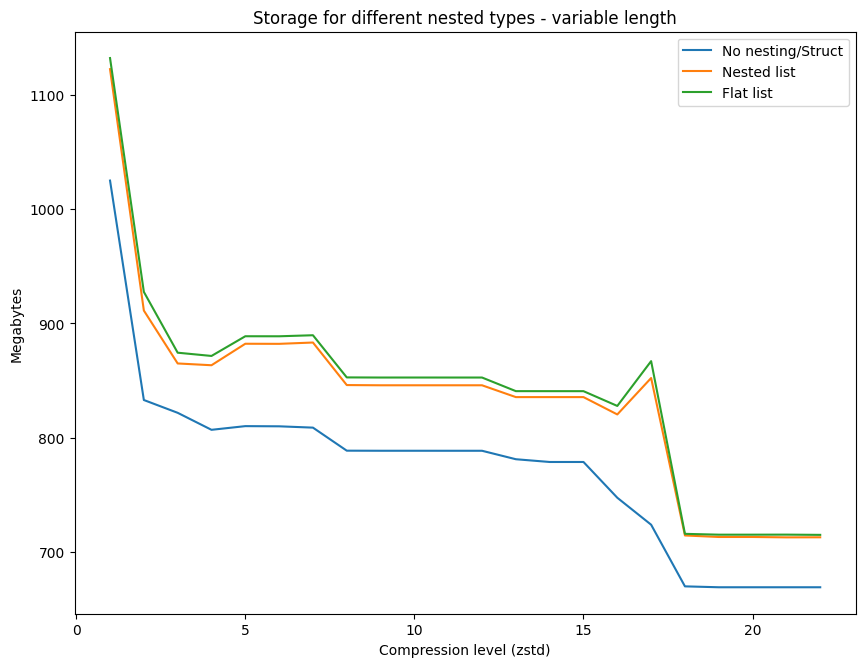
The chart is exactly the same as for the fixed length data, with the same curious peaks, and the same 3 trends that we see in the evolution of the compression level and size on disk.

Queries

To test the performance of queries on the nested data structures I used 3 different calculations that are common when dealing with order books. These aren’t the most complex calculations by a long shot, but they were chosen for the different operations they carry out on the columns. In each case, I assume that the data has not been sorted, either within the JSON files or during the ingest phase.

1. Mid-price & spread - mean of best bid & best ask, difference between best bid & best ask
   • finding maximum & minimum price information
2. Total queue imbalance - total volume of bids & asks weighted, indicating buying/selling pressure
   • summing all the volume on both bids & asks
3. Bid/ask depth at given level (I use ask depth @ 500) - sum of volume within price interval
   • selecting all ask prices between mid-price and 500 depth, then summing that volume

If we think back to our original JSON nested structure, the first 2 queries are operating on a single element within the inner array, while the third query is using both elements.

The 3 different queries for each nested structure are within lob_process_fix.py for the fixed length and lob_process_var.py for the variable length.

Query plans

The different nested structures require alternative syntax to run the 3 queries. Depending on the level of nesting this means either running expressions directly on the nested type, or using a combination of group_by() and agg() operations. Some of the syntax for queries operating on the nested structures could become slightly unwieldy, as they operate on the nested elements rather than columns. This isn’t really much of a problem for these relatively straightforward queries, but could pose a usability question in the case of more complex or sophisticated queries.

Visualisations produced with Graphviz using Polars’ handy show_graph() method are available in the appendix. I only reproduce those for the fixed length data for the sake of brevity. The aim is to illustrate the different queries to gain some insight into the query logic and any optimisations Polars carries out. Two of the queries are subject to optimisations by Polars, for the Mid-price & spread, where an additional with_columns() is used for the Flat array, Flat list and Struct to pull out the nested/composite elements, and for Ask depth at 500, with caching used for the join() operation for No nesting and Struct.

Results

Fixed length

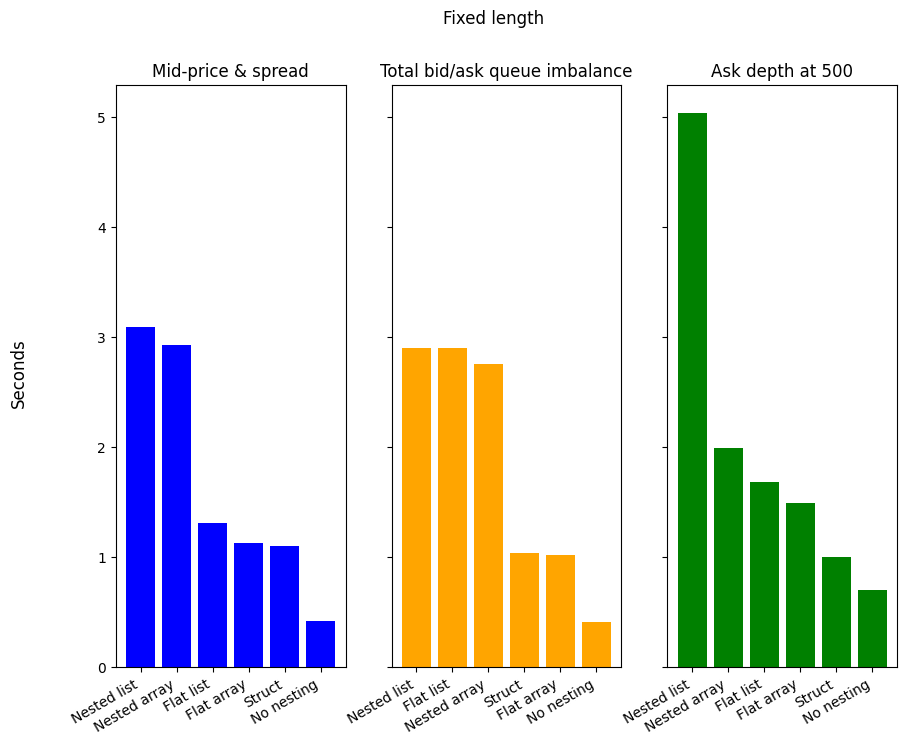
Structure	Mid-price & spread	Total bid/ask queue imbalance	Ask depth at 500
No nesting	0.4	0.4	0.7
Nested array	2.9	2.8	2.0
Flat array	1.1	1.0	1.5
Nested list	3.1	2.9	5.0
Flat list	1.3	2.9	1.7
Struct	1.1	1.0	1.0

No nesting offers superior performance across all 3 queries. It is 61.97% faster for Mid-price & spread, 59.81% for Total bid/ask queue imbalance, and 30.38% for the Ask depth at 500, as compared to the next fastest. Struct only really offers a gain over the nested types when taking the most complex query (Ask depth at 500) into account, otherwise, for Mid-price & spread and Total bid/ask queue imbalance it is more or less on par with Flat array. For all queries, both array versions are marginally faster than their list counterparts. The stand out structure is Nested list for the Ask depth at 500 query, since it is significantly slower than all others, in fact, compared to the same array version it is 152.67% slower. I recall here that this query relies on filtering, however, I don’t use filter() within the list namespace, since you can’t refer to a named column using list.eval() or list.agg(). The memory efficiency and performance of arrays over lists, as detailed in the Polars documentation, is evident in our queries, nevertheless, No nesting is the clear winner.

Variable length

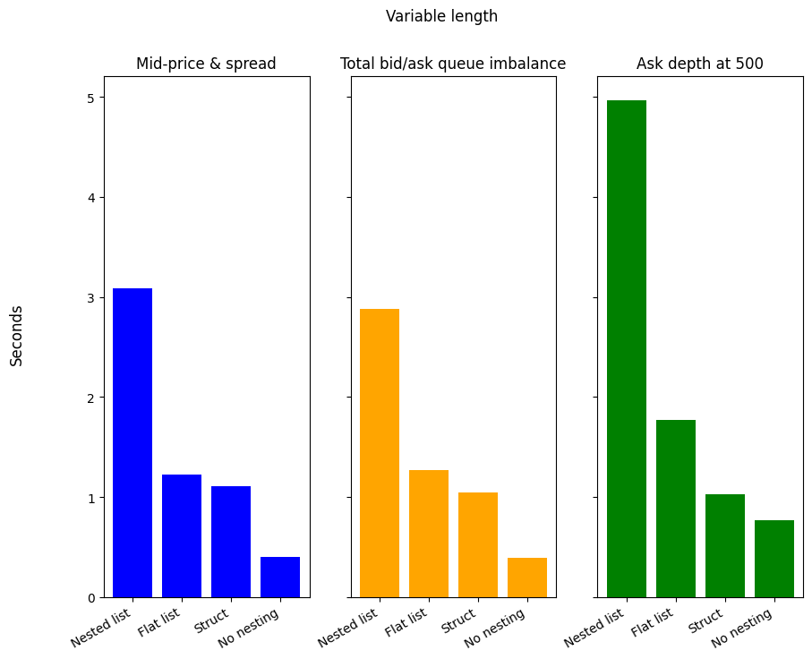
Structure	Mid-price & spread	Total bid/ask queue imbalance	Ask depth at 500
No nesting	0.4	0.4	0.8
Nested list	3.1	2.9	5.0
Flat list	1.2	1.3	1.8
Struct	1.1	1.0	1.0

No nesting also offers a clear speed advantage for the 3 queries acting on variable length data, being 63.88%, 61.97%, and 25.52% faster for Mid-price & spread, Total bid/ask queue imbalance, and Ask depth at 500, compared to the next fastest. In each case, Nested list is the slowest, followed by Flat list and Struct. In a similar way as for the fixed length data, Nested list shows the worst performance for Ask depth at 500, being 180.16% slower than Flat list. Overall, No nesting is the hands down winner, outpacing all the other structures.

Conclusion

So, to nest, or not to nest? Well, it depends. The results for ingesting JSON data show that using nested structures does offer a performance advantage for both fixed length and variable length data. Whereas for running queries to obtain various calculations from our data, nested types are detrimental. Using nested types is also penalising in terms of the storage requirements. Therefore, it becomes a judgement based on how frequently you are likely to be carrying out these tasks. Especially since the performance advantage for using nested types to ingest JSON data is smaller than the gain for queries on our dataframes without nesting. I think it is also relevant to think about the inherent structure of your data, and what sort of query structure it is likely to result in? Do the expressions within the array and list namespace suffice, or do you require something more complicated? Does your data lend itself naturally to using a series of nested eval or agg expressions against array or list elements, or are you adding a unnecessary layer of complexity?

I believe order book data provides a solid base from which to start answering this question, but there are limitations. The dataset only contains 4 variables, and further insights might be gained by adding further columns. It might also be possible to obtain the same performance advantage for ingesting JSON data using a library such as glom, which is designed to handle nested structures. Or, if you intend to run the same query on nested structures on a regular basis, it might be relevant to write a UDF or Rust plugin to maximise the performance. Finally, I’d also be very interested to see whether these results hold when expanding this dataset to bigger than memory, using Polars’ streaming functionality.

Thanks to those who attended the PyData talk, as well as those who asked questions or made remarks, whether online or in-person, for helping to make it participative. I’m happy to hear any further comments or feedback!

Appendix

Dataframes

To avoid repetition, I only reproduce df.head() for the fixed length data, since the structure of the columns is the same for the variable length data.

No nesting

+----------------+------------+----------+---------+----------+----------+
| last_update_id | timestamp  | bids_p   | bids_v  | asks_p   | asks_v   |
| ---            | ---        | ---      | ---     | ---      | ---      |
| u32            | u32        | f64      | f64     | f64      | f64      |
+========================================================================+
| 55075466       | 1757404800 | 70786.19 | 0.00497 | 70840.11 | 0.000185 |
| 55075466       | 1757404800 | 70786.2  | 0.00497 | 70840.12 | 0.000295 |
| 55075466       | 1757404800 | 70786.21 | 0.00497 | 70840.13 | 0.000324 |
| 55075466       | 1757404800 | 70786.22 | 0.00497 | 70840.14 | 0.000513 |
| 55075466       | 1757404800 | 70786.23 | 0.00497 | 70840.15 | 0.000594 |
+----------------+------------+----------+---------+----------+----------+

Nested array

+----------------+-----------------------------------+-----------------------------------+------------+
| last_update_id | bids                              | asks                              | timestamp  |
| ---            | ---                               | ---                               | ---        |
| u32            | array[f64, (5000, 2)]             | array[f64, (5000, 2)]             | u32        |
+=====================================================================================================+
| 55075466       | [[70786.19, 0.00497], [70786.2... | [[70840.11, 0.000185], [70840.... | 1757404800 |
| 55076350       | [[70775.56, 0.005469], [70775.... | [[70829.36, 0.000642], [70829.... | 1760587200 |
| 55077161       | [[70753.52, 0.005038], [70753.... | [[70807.86, 0.000668], [70807.... | 1763506800 |
| 55073749       | [[70784.32, 0.004542], [70784.... | [[70837.34, 0.000426], [70837.... | 1751223600 |
| 55069991       | [[70736.46, 0.005241], [70736.... | [[70790.38, 0.000126], [70790.... | 1737694800 |
+----------------+-----------------------------------+-----------------------------------+------------+

Flat array

+----------------+---------------------+----------------------+------------+
| last_update_id | bids                | asks                 | timestamp  |
| ---            | ---                 | ---                  | ---        |
| u32            | array[f64, 2]       | array[f64, 2]        | u32        |
+==========================================================================+
| 55075466       | [70786.19, 0.00497] | [70840.11, 0.000185] | 1757404800 |
| 55075466       | [70786.2, 0.00497]  | [70840.12, 0.000295] | 1757404800 |
| 55075466       | [70786.21, 0.00497] | [70840.13, 0.000324] | 1757404800 |
| 55075466       | [70786.22, 0.00497] | [70840.14, 0.000513] | 1757404800 |
| 55075466       | [70786.23, 0.00497] | [70840.15, 0.000594] | 1757404800 |
+----------------+---------------------+----------------------+------------+

Nested list

+----------------+-----------------------------------+-----------------------------------+------------+
| last_update_id | bids                              | asks                              | timestamp  |
| ---            | ---                               | ---                               | ---        |
| u32            | list[list[f64]]                   | list[list[f64]]                   | u32        |
+=====================================================================================================+
| 55075466       | [[70786.19, 0.00497], [70786.2... | [[70840.11, 0.000185], [70840.... | 1757404800 |
| 55076350       | [[70775.56, 0.005469], [70775.... | [[70829.36, 0.000642], [70829.... | 1760587200 |
| 55077161       | [[70753.52, 0.005038], [70753.... | [[70807.86, 0.000668], [70807.... | 1763506800 |
| 55073749       | [[70784.32, 0.004542], [70784.... | [[70837.34, 0.000426], [70837.... | 1751223600 |
| 55069991       | [[70736.46, 0.005241], [70736.... | [[70790.38, 0.000126], [70790.... | 1737694800 |
+----------------+-----------------------------------+-----------------------------------+------------+

Flat list

+----------------+---------------------+----------------------+------------+
| last_update_id | bids                | asks                 | timestamp  |
| ---            | ---                 | ---                  | ---        |
| u32            | list[f64]           | list[f64]            | u32        |
+==========================================================================+
| 55075466       | [70786.19, 0.00497] | [70840.11, 0.000185] | 1757404800 |
| 55075466       | [70786.2, 0.00497]  | [70840.12, 0.000295] | 1757404800 |
| 55075466       | [70786.21, 0.00497] | [70840.13, 0.000324] | 1757404800 |
| 55075466       | [70786.22, 0.00497] | [70840.14, 0.000513] | 1757404800 |
| 55075466       | [70786.23, 0.00497] | [70840.15, 0.000594] | 1757404800 |
+----------------+---------------------+----------------------+------------+

Struct

+----------------+------------+--------------------+---------------------+
| last_update_id | timestamp  | bids               | asks                |
| ---            | ---        | ---                | ---                 |
| u32            | u32        | struct[2]          | struct[2]           |
+========================================================================+
| 55075466       | 1757404800 | {70786.19,0.00497} | {70840.11,0.000185} |
| 55075466       | 1757404800 | {70786.2,0.00497}  | {70840.12,0.000295} |
| 55075466       | 1757404800 | {70786.21,0.00497} | {70840.13,0.000324} |
| 55075466       | 1757404800 | {70786.22,0.00497} | {70840.14,0.000513} |
| 55075466       | 1757404800 | {70786.23,0.00497} | {70840.15,0.000594} |
+----------------+------------+--------------------+---------------------+

Query plan visualisation

Mid-price & spread

No nesting

Nested array

Flat array

Nested list

Flat list

Struct

Total queue imbalance

No nesting

Nested array

Flat array

Nested list

Flat list

Struct

Ask depth at 500

No nesting

Nested array

Flat array

Nested list

Flat list

Struct