ARDL: Replication of eViews example on bond term structure in R package
In this first blog post I thought it would be relevant to publish something about Autoregressive Distributed Lag (ARDL) models and the bounds testing approach for cointegration (Pesaran, Shin & Smith, 2001). I discovered these models a few years ago, and, in particular, have become a big fan of the excellent ARDL package from Kleanthis Natsiopoulos for R. What is special about the ARDL package is replication of the original empirical application in the PSS paper, which you can read about in ARDL bounds test for cointegration: Replicating the Pesaran et al. (2001) results for the UK earnings equation using R (Natsiopoulos & Tzeremes, 2022).
So the ARDL package doesn’t need to prove itself by any further replication, but do the results it produces stack up against other econometric software? This is a post replicating results from eViews, using an example analysing the term structure of Canadian interest rates and the ARDL package. The example forms part of a comprehensive series of posts on the eViews blog (Part 1, Part 2), explaining the theory behind ARDL and the bounds test for cointegration. These posts - alongside Dave Giles’ excellent blogs (here, here, and here) - are great resources for learning more about ARDL modelling and cointegration. But we don’t necessarily need to use eViews. The goal of this post is to demonstrate that we can get materially the same results using open source econometrics packages compared to commercially available software.
First, let’s load the packages we’ll use, configure our locale, and turn off scientific notation (just a preference of mine).
library(hexView)
library(knitr)
library(CADFtest)
library(lmtest)
library(ARDL)
library(tidyr)
library(ggplot2)
library(broom)
library(sandwich)

Sys.setlocale("LC_TIME", "en_GB.UTF-8")
options(scipen=999)
Data
The eViews example uses data originally sourced from the Canadian Socioeconomic Database from Statistics Canada (CANSIM), with the following maturities:
Treasury Bill
- 1 month
TBILL1M - 3 months
TBILL3M - 6 months
TBILL6M - 1 year
TBILL1Y
Treasury Notes
- 2 years
BBY2Y - 5 years
BBY5Y - 10 years
BBY10Y
You can get equivalent data from the Bank of
Canada, but we use
the provided eViews workfile, ardl.example.WF1, which contains exactly
the same data in the example, with 196 observations on a monthly
frequency from January 2001 to April 2017. It is currently available on
the eViews website
here.
We import the data using the readEViews function from the hexView
package, remove unnecessary columns, and trim the start and end of the
series.
data <- readEViews("ardl.example.WF1", as.data.frame = TRUE)
maturities <- c('TBILL1M', 'TBILL3M', 'TBILL6M', 'TBILL1Y', 'BBY2Y', 'BBY5Y', 'BBY10Y')
data <- data[, c('Date', maturities)]
data$Date <- as.Date(data$Date)
data <- data[data$Date >= "2001-01-01" & data$Date <= "2017-04-01", ]
data[, maturities] <- round(data[, maturities], 2)
kable(head(data, 5), format = "html", digits = 2, row.names = FALSE)
| Date | TBILL1M | TBILL3M | TBILL6M | TBILL1Y | BBY2Y | BBY5Y | BBY10Y |
|---|---|---|---|---|---|---|---|
| 2001-01-01 | 5.17 | 5.11 | 5.00 | 4.90 | 4.88 | 5.14 | 5.39 |
| 2001-02-01 | 5.04 | 4.87 | 4.80 | 4.79 | 4.81 | 5.09 | 5.36 |
| 2001-03-01 | 4.70 | 4.58 | 4.52 | 4.52 | 4.69 | 5.03 | 5.41 |
| 2001-04-01 | 4.56 | 4.43 | 4.40 | 4.45 | 4.76 | 5.23 | 5.66 |
| 2001-05-01 | 4.32 | 4.34 | 4.41 | 4.55 | 4.99 | 5.61 | 5.96 |
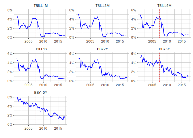
Visualisation
Let’s replicate the graphs for the different maturities, including a red vertical line indicating a structural break for the start of the US global financial crisis. We also create a dummy variable to indicate its presence for our models.
data_long <- data %>% pivot_longer(cols=all_of(maturities),
                    names_to='instrument',
                    values_to='yield')
ggplot(data=data_long, aes(x=Date, y=yield)) +
  geom_line(color = "blue") +
  # Use a factor here to control ordering of graphs in facet
  facet_wrap( ~ factor(instrument, levels=maturities), ncol = 3, axes = 'all') +
  scale_y_continuous(labels = scales::percent_format(scale = 1)) +
  labs(x = "", y = "") +
  geom_vline(
    xintercept=as.Date('2007-07-04'),
    linetype='dashed',
    color='red',
    linewidth=0.25) +
  theme(panel.background = element_rect(fill = "white", colour = "white"),
        panel.grid.major = element_line(colour = "grey"),
        panel.grid.minor = element_line(colour = "grey"),
        strip.background =element_rect(fill="white"))
#Create dummy variable for financial crisis.
data$dum0708 <- ifelse(data$Date > '2007-06-01', 1, 0)
Unit root tests
Next, we test the order of integration to ensure that none of the
variables are integrated of order 2 or higher ($I(2)$). The eViews
example uses an Augmented
Dickey–Fuller
(ADF) test, including an intercept and selection of lag length based on
the Schwarz Information
Criterion.
The CADFtest
package is
used to carry out the test in R.
adf_tests <- lapply(maturities, function(maturity) {
  y <- diff(data[,maturity], differences = 1)
  # Drift corresponds to intercept, we use y ~ 1 to carry out ordinary ADF
  adf <- CADFtest(y ~ 1, type = "drift", max.lag.y = 14, criterion = "BIC")
  return (list(
    series = maturity,
    prob = format(round(adf$p.value), nsmall = 2),
    lag = adf$max.lag.y,
    max_lag = 14
  ))
})

kable(
  data.frame(t(sapply(adf_tests,c))),
  caption = "ADF test results",
  format = "html",
  row.names = FALSE,
  col.names = c("Series", "Prob", "Lag", "Max Lag")
  )
| Series | Prob | Lag | Max Lag |
|---|---|---|---|
| TBILL1M | 0.00 | 2 | 14 |
| TBILL3M | 0.00 | 1 | 14 |
| TBILL6M | 0.00 | 1 | 14 |
| TBILL1Y | 0.00 | 0 | 14 |
| BBY2Y | 0.00 | 0 | 14 |
| BBY5Y | 0.00 | 0 | 14 |
| BBY10Y | 0.00 | 0 | 14 |
Our results mirror those calculated by eViews, with the exception that
CADFtest selects no lags for TBILL1Y, as opposed to 1 lag.
ARDL Bounds Testing
After determining that none of the series are $I(2)$, we can begin the ARDL bounds testing procedure for cointegration. The example uses 3 models with different dependent/independent variables and deterministic specification:
| Model | Dependent variable | Independent variable(s) | Deterministic terms |
|---|---|---|---|
| 1 | BBY10Y |
TBILL1M |
Restricted constant |
| 2 | TBILL6M |
TBILL3M, TBILL1M |
Unrestricted constant |
| 3 | BBY2Y |
TBILL1Y, TBILL1M |
Unrestricted constant |
Model 1: No cointegrating relationship
To start with we need to choose a lag order for our model. The ARDL
package provides an auto_ardl function to carry out automatic
selection in a similar fashion to eViews, according to different
information criterion. We use the Akaike Information Criteria (AIC) and
a maximum of 4 lags, as in the example.
lag_select_1 <- auto_ardl(
  BBY10Y ~ TBILL1M | dum0708,
  data = data,
  max_order = 4,
  selection = "AIC",
  grid = TRUE
  )
kable(
  data.frame(t(sapply(lag_select_1$best_order,c))),
  format = "html",
  row.names = FALSE
  )
| BBY10Y | TBILL1M |
|---|---|
| 1 | 3 |
The automatic selection picks exactly the same lag specification as the eViews example: $ARDL(1,3)$. Now, we can estimate the model.
ardl_13 <- ardl(
  BBY10Y ~ TBILL1M | dum0708,
  data = data,
  order = lag_select_1$best_order
  )

reg_table_cols <- c(
  'Variable',
  'Coefficient',
  'Std. Error',
  't-Statistic',
  'Prob'
  )

kable(
  tidy(ardl_13)[c(2,3,4,5,6,7,1),],
  caption = "Dependent Variable BBY10Y",
  col.names = reg_table_cols,
  digits = 4
)
| Variable | Coefficient | Std. Error | t-Statistic | Prob |
|---|---|---|---|---|
| L(BBY10Y, 1) | 0.9517 | 0.0191 | 49.9014 | 0.0000 |
| TBILL1M | 0.2523 | 0.0699 | 3.6087 | 0.0004 |
| L(TBILL1M, 1) | -0.3816 | 0.0940 | -4.0605 | 0.0001 |
| L(TBILL1M, 2) | 0.0190 | 0.0939 | 0.2028 | 0.8395 |
| L(TBILL1M, 3) | 0.1207 | 0.0674 | 1.7908 | 0.0749 |
| dum0708 | -0.0988 | 0.0509 | -1.9405 | 0.0538 |
| (Intercept) | 0.1835 | 0.0867 | 2.1154 | 0.0357 |
Dependent Variable BBY10Y
glanced <- t(glance(ardl_13)[,c(1,2,3,7,4,5)])
reg_validation_rows <- c(
  'R-squared',
  'Adjusted R-squared',
  'S.E. of regression',
  'Log likelihood',
  'F-statistic',
  'Prob(F-statistic)')
rownames(glanced) <- reg_validation_rows

kable(glanced, digits = 4)
| R-squared | 0.9803 |
| Adjusted R-squared | 0.9796 |
| S.E. of regression | 0.1888 |
| Log likelihood | 51.4742 |
| F-statistic | 1538.6296 |
| Prob(F-statistic) | 0.0000 |
The results are very close to the eViews example. I won’t do a
side-by-side comparison, but, for example, if we take the coefficient
for the intercept, eViews estimates 0.180150 and the ARDL package
estimates 0.18349, with p-values of 0.0376 versus 0.035724.
The next step is to check whether the residuals from the model are serially correlated, so we use the Breusch-Godfrey test from the lmtest package. We provide results for both the $\chi^2$ and $F$ test, using 2 lags as in eViews.
bg_f <- bgtest(ardl_13, order = 2, type = "F")
bg_chi <- bgtest(ardl_13, order = 2, type = "Chisq")

kable(
  data.frame(
    test = c('F test', 'Chi-squared'),
    statistic = c(bg_f$statistic, bg_chi$statistic),
    p_value = c(bg_f$p.value, bg_chi$p.value)
  ),
  caption = "Breusch-Godrey Serial Correlation LM Test",
  format = "html",
  row.names = FALSE,
  col.names = c('', 'Statistic', 'Prob.')
)
| Statistic | Prob. | |
|---|---|---|
| F test | 0.3844223 | 0.6813894 |
| Chi-squared | 0.8030954 | 0.6692834 |
In both cases, with the $\chi^2$ test statistic p-value and $F$ test
statistic p-value, we can’t reject the null hypothesis, as in eViews,
and therefore conclude that the residuals are serially uncorrelated.
eViews denotes the Chi-squared test statistic as Obs*R-squared. The
results aren’t exactly the same, but the conclusion is the same.
Additionally, we need to check for heteroskedasticity in the residuals,
so once again following the example, we use the Breusch-Pagan test also
from the lmtest package.
bp <- bptest(ardl_13)

kable(
  data.frame(
    statistic = c(bp$statistic),
    p_value = c(bp$p.value)
  ),
  caption = "Heteroskedasticity Test: Breusch-Pagan-Godfrey",
  format = "html",
  row.names = FALSE,
  col.names = c('Statistic', 'Prob.')
)
| Statistic | Prob. |
|---|---|
| 10.29698 | 0.1126898 |
We only have the $\chi^2$ test statistic p-value with bptest, but it
corroborates the results from eViews - the residuals from the model are
homoskedastic.
Once we have ruled out serial correlation and heteroskedasticity, we can
proceed to the bounds test. We set the case to 2, corresponding to
“Restricted intercept and no trend”, and run the test for the different
significance levels reported in eViews.
levels_eq <- multipliers(ardl_13, type = "lr", se = TRUE)
kable(
  levels_eq[c(2,1),],
  caption = "Levels Equation",
  format = "html",
  digits = 4,
  row.names = FALSE,
  col.names = reg_table_cols
  )
| Variable | Coefficient | Std. Error | t-Statistic | Prob |
|---|---|---|---|---|
| TBILL1M | 0.2156 | 0.3290 | 0.6554 | 0.5130 |
| (Intercept) | 3.7970 | 1.0622 | 3.5748 | 0.0004 |
sig_levels <- c(0.1, 0.05, 0.025, 0.01)

f_bounds_tests <- lapply(sig_levels, function(sig_level) {
  bounds_test <- bounds_f_test(ardl_13, case = 2, alpha = sig_level)
  list(
    f_statistic = round(unname(bounds_test$statistic), 4),
    signif = paste(sig_level * 100, "%", sep = ''),
    I_0 = round(bounds_test[["parameters"]][["Lower-bound I(0)"]], 4),
    I_1 = round(bounds_test[["parameters"]][["Upper-bound I(1)"]], 4)
  )
})

f_bounds_results_cols <- c('F-statistic', 'Signif.', 'I(0)', 'I(1)')

kable(
  data.frame(t(sapply(f_bounds_tests,c))),
  caption = "F-Bounds Test",
  format = "html",
  row.names = FALSE,
  col.names = f_bounds_results_cols
  )
| F-statistic | Signif. | I(0) | I(1) |
|---|---|---|---|
| 2.2754 | 10% | 3.0213 | 3.5032 |
| 2.2754 | 5% | 3.6209 | 4.1351 |
| 2.2754 | 2.5% | 4.1988 | 4.7444 |
| 2.2754 | 1% | 4.9437 | 5.5629 |
The results of the F-Bounds test align with those from eViews, with a $F$ test statistic that is below the $I(0)$ critical bound for all significance levels.
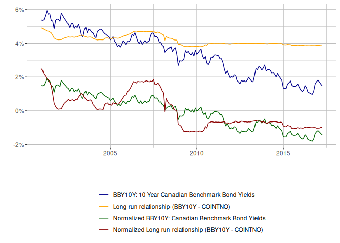
eViews also presents the results of long-run relationship, which we can
calculate using the multipliers function.
The estimated long-run relationship is very close to eViews, but since we haven’t got evidence for cointegration it isn’t valid. And we can see this from the fit, if we reproduce the chart provided by eViews.
lr_fit <- data.frame(
  Date = data$Date,
  BBY10Y = data$BBY10Y,
  COINT = coint_eq(ardl_13, case = 2)
)
# Create the normalized series
normalized <- scale(lr_fit[,c('BBY10Y', 'COINT')])
lr_fit$norm_BBY10Y <- normalized[,'BBY10Y']
lr_fit$norm_COINT <- normalized[, 'COINT']

lr_fit %>%
  pivot_longer(cols=c('BBY10Y', 'COINT', 'norm_BBY10Y', 'norm_COINT'),
               names_to='series',
               values_to = 'value') %>%
  ggplot(aes(x=Date, y=value, group = series, color = series)) +
    geom_line() +
    scale_color_manual(name='', labels=c(
      'BBY10Y: 10 Year Canadian Benchmark Bond Yields',
      'Long run relationship (BBY10Y - COINTNO)',
      'Normalized BBY10Y: Canadian Benchmark Bond Yields',
      'Normalized Long run relationship (BBY10Y - COINTNO)'
      ),
      values=c('darkblue', 'orange', 'darkgreen', 'darkred')) +
      scale_y_continuous(labels = scales::percent_format(scale = 1)) +
      labs(x = "", y = "") +
      geom_vline(
        xintercept=as.Date('2007-06-01'),
        linetype='dashed',
        color='red',
        linewidth=0.25) +
      theme(panel.background = element_rect(fill = "white", colour = "white"),
          panel.grid.major = element_line(colour = "grey"),
          panel.grid.minor = element_line(colour = "grey"),
          strip.background =element_rect(fill="white"),
          legend.position = 'bottom',
          legend.direction = 'vertical')
Model 2: Usual Cointegrating Relationship
The example skips steps here with the lag order selection, but they end up with a $ARDL(6,6,3)$ model, having identified problems with both serial correlation and heteroskedasticity. The final model they use doesn’t have serial correlation, but requires an adjustment for Heteroskedasticity-consistent standard errors.
Notably, this model uses Case 3 with “Unrestricted intercept and no trend”, which means the constant won’t enter the levels relationship. Let’s estimate it and run the same tests on the final model.
ardl_663 <- ardl(TBILL6M ~ TBILL3M + TBILL1M | dum0708, data = data, order = c(6,6,3))

bg_f_663 <- bgtest(ardl_663, order = 2, type = "F")
bg_chi_663 <- bgtest(ardl_663, order = 2, type = "Chisq")

kable(
  data.frame(
    test = c('F test', 'Chi-squared'),
    statistic = c(bg_f_663$statistic, bg_chi_663$statistic),
    p_value = c(bg_f_663$p.value, bg_chi_663$p.value)
  ),
  caption = "Breusch-Godrey Serial Correlation LM Test",
  format = "html",
  row.names = FALSE,
  digits = 4,
  col.names = c('', 'Statistic', 'Prob.')
)
| Statistic | Prob. | |
|---|---|---|
| F test | 1.1060 | 0.3333 |
| Chi-squared | 2.4547 | 0.2931 |
bp_663 <- bptest(ardl_663)

kable(
  data.frame(
    statistic = c(bp_663$statistic),
    p_value = c(bp_663$p.value)
  ),
  caption = "Heteroskedasticity Test: Breusch-Pagan-Godfrey",
  format = "html",
  row.names = FALSE,
  digits = 4,
  col.names = c('Statistic', 'Prob.'))
| Statistic | Prob. |
|---|---|
| 68.7467 | 0 |
Results for the $ARDL(6,6,3)$ model are very similar to the eViews
example, with no serial correlation. It applies a Heteroskedasticity and
Autocorrelation Consistent (HAC) covariance matrix using the Hewey-West
estimator to deal with the lack of homoskedasticity in the residuals. We
can do the same using the HeweyWest function from the
sandwich
package, which we can pass to the functions within the ardl package.
Notably, for the levels equation, we provide the same formula to the
multipliers function, but without the intercept, since we’re using
Case 3.
# Re-estimate without intercept for LR multipliers
ardl_663_nc <- ardl(
  TBILL6M ~ TBILL3M + TBILL1M -1 | dum0708,
  data = data,
  order = c(6,6,3))
levels_eq <- multipliers(ardl_663_nc,
                         type = "lr",
                         vcov_matrix = NeweyWest(
                           ardl_663_nc,
                           adjust = TRUE,
                           prewhite = TRUE
                           ),
                         se = TRUE)
kable(
  levels_eq,
  caption = "Levels Equation",
  format = "html",
  row.names = FALSE,
  col.names = reg_table_cols,
  digits = 4
  )
| Variable | Coefficient | Std. Error | t-Statistic | Prob |
|---|---|---|---|---|
| TBILL3M | 2.0408 | 0.1894 | 10.7724 | 0 |
| TBILL1M | -1.0426 | 0.1950 | -5.3453 | 0 |
f_bounds_tests <- lapply(sig_levels, function(sig_level) {
  f_bounds_test <- bounds_f_test(ardl_663,
                                 case = 3,
                                 alpha = sig_level,
                                 vcov_matrix = NeweyWest(
                                   ardl_663,
                                   adjust = TRUE,
                                   prewhite = TRUE))
  list(
    f_statistic = unname(f_bounds_test$statistic),
    signif = paste(sig_level * 100, "%", sep = ''),
    I_0 = f_bounds_test[["parameters"]][["Lower-bound I(0)"]],
    I_1 = f_bounds_test[["parameters"]][["Upper-bound I(1)"]]
  )
})

t_bounds_tests <- lapply(sig_levels, function(sig_level) {
  t_bounds_test <- bounds_t_test(ardl_663,
                                 case = 3,
                                 alpha = sig_level,
                                 vcov_matrix = NeweyWest(
                                   ardl_663,
                                   adjust = TRUE,
                                   prewhite = TRUE))
  list(
    f_statistic = unname(t_bounds_test$statistic),
    signif = paste(sig_level * 100, "%", sep = ''),
    I_0 = t_bounds_test[["parameters"]][["Lower-bound I(0)"]],
    I_1 = t_bounds_test[["parameters"]][["Upper-bound I(1)"]]
  )
})

t_bounds_results_cols <- c('t-statistic', 'Signif.', 'I(0)', 'I(1)')

kable(
  data.frame(t(sapply(f_bounds_tests,c))),
  digits = 2,
  caption = "F-Bounds Test",
  format = "html",
  row.names = FALSE,
  col.names = f_bounds_results_cols
)
| F-statistic | Signif. | I(0) | I(1) |
|---|---|---|---|
| 10.07415 | 10% | 3.164478 | 4.098948 |
| 10.07415 | 5% | 3.790645 | 4.806771 |
| 10.07415 | 2.5% | 4.393914 | 5.461954 |
| 10.07415 | 1% | 5.165538 | 6.337465 |
kable(
  data.frame(t(sapply(t_bounds_tests,c))),
  digits = 2,
  caption = "t-Bounds Test",
  format = "html",
  row.names = FALSE,
  col.names = t_bounds_results_cols
)
| t-statistic | Signif. | I(0) | I(1) |
|---|---|---|---|
| -5.183061 | 10% | -2.562839 | -3.192939 |
| -5.183061 | 5% | -2.86012 | -3.507306 |
| -5.183061 | 2.5% | -3.114437 | -3.786882 |
| -5.183061 | 1% | -3.424963 | -4.097248 |
The coefficients for the long-run relationship are very close and both bounds tests indicate that we have evidence for cointegration, as demonstrated in the eViews modelling. The standard errors in the long-run estimation and test statistics in the bounds tests are slightly different from eViews, probably owing to the HAC adjustment. Now, time to visualise the fit.
lr_fit <- data.frame(
  Date = data$Date,
  TBILL6M = data$TBILL6M,
  COINTNONDEG = coint_eq(ardl_663, case = 3)
)
# Create the normalized series
normalized <- scale(lr_fit[,c('TBILL6M', 'COINTNONDEG')])
lr_fit$norm_TBILL6M <- normalized[,'TBILL6M']
lr_fit$norm_COINTNONDEG <- normalized[, 'COINTNONDEG']

lr_fit %>%
  pivot_longer(cols=c(
    'TBILL6M',
    'COINTNONDEG',
    'norm_TBILL6M',
    'norm_COINTNONDEG'),
                names_to='series',
                values_to = 'value') %>%
  ggplot(aes(x=Date, y=value, color = series)) +
    geom_line() +
    scale_color_manual(name='', labels=c(
      'TBILL6M: 6 Month Canadian T-Bill Yields',
      'Long run relationship (TBILL6M - COINTNONDEG)',
      'Normalized TBILL6M: 6 Month Canadian T-Bill Yields',
      'Normalized Long run relationship (TBILL6M - COINTNONDEG)'
      ),
      values=c('darkblue', 'orange', 'darkgreen', 'darkred'),
      limits=c('TBILL6M', 'COINTNONDEG', 'norm_TBILL6M', 'norm_COINTNONDEG')) +
    scale_y_continuous(labels = scales::percent_format(scale = 1),
                       breaks = c(-2, -1, 0, 1, 2, 3, 4, 5, 6)) +
    labs(x = "", y = "") +
    geom_vline(
      xintercept=as.Date('2007-06-01'),
      linetype='dashed',
      color='red',
      linewidth=0.25) +
    theme(panel.background = element_rect(fill = "white", colour = "white"),
          panel.grid.major = element_line(colour = "grey"),
          panel.grid.minor = element_line(colour = "grey"),
          strip.background =element_rect(fill="white"),
          legend.position = "bottom",
          legend.direction = "vertical")
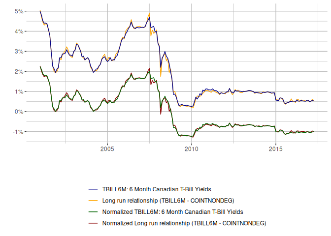
The fit is good. We can now also examine the RECM and speed of adjustment.
recm_663 <- recm(ardl_663, case = 3)

kable(
  tidy(recm_663),
  caption = "ECM Regression",
  col.names = reg_table_cols,
  digits = 4
)
| Variable | Coefficient | Std. Error | t-Statistic | Prob |
|---|---|---|---|---|
| (Intercept) | -0.0106 | 0.0072 | -1.4661 | 0.1444 |
| d(L(TBILL6M, 1)) | 0.1001 | 0.0992 | 1.0086 | 0.3146 |
| d(L(TBILL6M, 2)) | 0.2175 | 0.0887 | 2.4504 | 0.0153 |
| d(L(TBILL6M, 3)) | 0.1607 | 0.0798 | 2.0143 | 0.0455 |
| d(L(TBILL6M, 4)) | -0.1152 | 0.0785 | -1.4676 | 0.1440 |
| d(L(TBILL6M, 5)) | -0.1951 | 0.0716 | -2.7249 | 0.0071 |
| d(TBILL3M) | 1.2445 | 0.0701 | 17.7455 | 0.0000 |
| d(L(TBILL3M, 1)) | -0.0941 | 0.1707 | -0.5514 | 0.5821 |
| d(L(TBILL3M, 2)) | -0.4430 | 0.1326 | -3.3404 | 0.0010 |
| d(L(TBILL3M, 3)) | -0.1581 | 0.0786 | -2.0112 | 0.0459 |
| d(L(TBILL3M, 4)) | 0.0438 | 0.0714 | 0.6141 | 0.5400 |
| d(L(TBILL3M, 5)) | 0.1846 | 0.0618 | 2.9851 | 0.0032 |
| d(TBILL1M) | -0.4080 | 0.0708 | -5.7594 | 0.0000 |
| d(L(TBILL1M, 1)) | 0.0262 | 0.0963 | 0.2722 | 0.7858 |
| d(L(TBILL1M, 2)) | 0.2543 | 0.0765 | 3.3253 | 0.0011 |
| dum0708 | 0.0189 | 0.0098 | 1.9353 | 0.0546 |
| ect | -0.5632 | 0.1018 | -5.5296 | 0.0000 |
ECM Regression
glanced <- t(glance(recm_663)[,c(1,2,3,7,4,5)])

rownames(glanced) <- reg_validation_rows

kable(glanced, digits = 4)
| R-squared | 0.9100 |
| Adjusted R-squared | 0.9017 |
| S.E. of regression | 0.0587 |
| Log likelihood | 278.0104 |
| F-statistic | 109.3339 |
| Prob(F-statistic) | 0.0000 |
With the ardl package we get an Error Correction Term (ECT) of -0.56
versus -0.54, so very close. All the other coefficients are also very
similar, for instance, $\Delta{TBILL3}_t$ is 1.24 in R, compared to
1.26 in eViews.
Model 3: Nonsensical Cointegrating Relationship
Finally, we consider BBY2Y as the dependent variable, with TBILL1Y
and TBILL1M as our independent variables. Again, we use Case 3. The
blog posts skips lag selection, and there is no indication what lag
order they use, so we’ll rely on the auto_ardl function using AIC as
our selection criteria. Obviously, without knowing what lag order was
used our results may differ more considerably.
lag_select_3 <- auto_ardl(
  BBY2Y ~ TBILL1Y + TBILL1M | dum0708,
  data = data,
  max_order = 4,
  selection = "AIC",
  grid = TRUE)
kable(
  data.frame(t(sapply(lag_select_3$best_order,c))),
  format = "html",
  row.names = FALSE
  )
| BBY2Y | TBILL1Y | TBILL1M |
|---|---|---|
| 3 | 3 | 3 |
So, the best lag order is $ARDL(3,3,3)$. We’ll continue on to the estimation of the model, then tests of serial correlation and heteroskedasticity.
ardl_333 <- ardl(
  BBY2Y ~ TBILL1Y + TBILL1M | dum0708,
  data = data,
  order = lag_select_3$best_order
  )

bg_f <- bgtest(ardl_333, order = 2, type = "F")
bg_chi <- bgtest(ardl_333, order = 2, type = "Chisq")

kable(
  data.frame(
    test = c('F test', 'Chi-squared'),
    statistic = c(bg_f$statistic, bg_chi$statistic),
    p_value = c(bg_f$p.value, bg_chi$p.value)
  ),
  caption = "Breusch-Godrey Serial Correlation LM Test",
  format = "html",
  row.names = FALSE,
  col.names = c('', 'Statistic', 'Prob.')
)
| Statistic | Prob. | |
|---|---|---|
| F test | 0.0949428 | 0.9094709 |
| Chi-squared | 0.2056679 | 0.9022768 |
bp <- bptest(ardl_333)

kable(
  data.frame(
    statistic = c(bp$statistic),
    p_value = c(bp$p.value)
  ),
  caption = "Heteroskedasticity Test: Breusch-Pagan-Godfrey",
  format = "html",
  row.names = FALSE,
  col.names = c('Statistic', 'Prob.')
)
| Statistic | Prob. |
|---|---|
| 32.50877 | 0.0011543 |
Replicating the results from eViews, we have no problem with serial correlation, but the residuals are heteroskedastic, so we apply a corrected-covariance matrix to the bounds tests and estimation of levels relationship.
ardl_333_nc <- ardl(
  BBY2Y ~ TBILL1Y + TBILL1M -1 | dum0708,
  data = data,
  order = lag_select_3$best_order
  )
levels_eq <- multipliers(ardl_333_nc,
                         type = "lr",
                         vcov_matrix = NeweyWest(
                           ardl_333_nc,
                           adjust = TRUE,
                           prewhite = TRUE),
                         se = TRUE)
kable(
  levels_eq,
  caption = "Levels Equation",
  format = "html",
  row.names = FALSE,
  col.names = reg_table_cols,
  digits = 4
)
| Variable | Coefficient | Std. Error | t-Statistic | Prob |
|---|---|---|---|---|
| TBILL1Y | 0.1286 | 1.1836 | 0.1086 | 0.9136 |
| TBILL1M | 0.9643 | 1.2806 | 0.7530 | 0.4524 |
The coefficients in the levels relationship are quite different from
eViews. Taking $TBILL1Y_t$, it is 0.13 in R, compared to 0.29 in
eViews. This is the first time we’ve seen such a considerable difference
in the results from ardl, and as previously mentioned is probably due
to the lag order selection.
We now replicate the bounds testing.
f_bounds_tests <- lapply(sig_levels, function(sig_level) {
  f_bounds_test <- bounds_f_test(ardl_333,
                                 case = 3,
                                 alpha = sig_level,
                                 vcov_matrix = NeweyWest(
                                   ardl_333,
                                   adjust = TRUE,
                                   prewhite = TRUE)
                                 )
  list(
    f_statistic = unname(f_bounds_test$statistic),
    signif = paste(sig_level * 100, "%", sep = ''),
    I_0 = f_bounds_test[["parameters"]][["Lower-bound I(0)"]],
    I_1 = f_bounds_test[["parameters"]][["Upper-bound I(1)"]]
  )
})

t_bounds_tests <- lapply(sig_levels, function(sig_level) {
  t_bounds_test <- bounds_t_test(ardl_333,
                                 case = 3,
                                 alpha = sig_level,
                                 vcov_matrix = NeweyWest(
                                   ardl_333,
                                   adjust = TRUE,
                                   prewhite = TRUE)
                                 )
  list(
    f_statistic = unname(t_bounds_test$statistic),
    signif = paste(sig_level * 100, "%", sep = ''),
    I_0 = t_bounds_test[["parameters"]][["Lower-bound I(0)"]],
    I_1 = t_bounds_test[["parameters"]][["Upper-bound I(1)"]]
  )
})

kable(
  data.frame(t(sapply(f_bounds_tests,c))),
  caption = "F-Bounds Test",
  digits = 2,
  format = "html",
  row.names = FALSE,
  col.names = f_bounds_results_cols
  )
| F-statistic | Signif. | I(0) | I(1) |
|---|---|---|---|
| 4.833843 | 10% | 3.164478 | 4.098948 |
| 4.833843 | 5% | 3.790645 | 4.806771 |
| 4.833843 | 2.5% | 4.393914 | 5.461954 |
| 4.833843 | 1% | 5.165538 | 6.337465 |
kable(
  data.frame(t(sapply(t_bounds_tests,c))),
  caption = "t-Bounds Test",
  digits = 2,
  format = "html",
  row.names = FALSE,
  col.names = t_bounds_results_cols
  )
| t-statistic | Signif. | I(0) | I(1) |
|---|---|---|---|
| -1.989419 | 10% | -2.562839 | -3.192939 |
| -1.989419 | 5% | -2.86012 | -3.507306 |
| -1.989419 | 2.5% | -3.114437 | -3.786882 |
| -1.989419 | 1% | -3.424963 | -4.097248 |
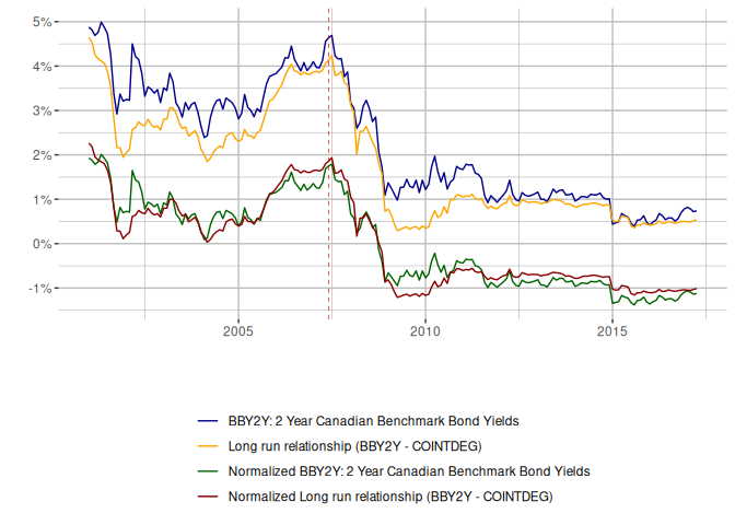
Despite the previous results with considerably different coefficients in the long-run multipliers, the F-bounds and t-bounds results are similar in substance to eViews. We have evidence for cointegration at the 5% level in the F-bounds tests, however, the t-bounds results lead us to determine that this is a nonsensical relationship.
We can see a poor fit in the cointegrating relationship.
lr_fit <- data.frame(
  Date = data$Date,
  BBY2Y = data$BBY2Y,
  COINTDEG = coint_eq(ardl_333, case = 3)
)
# Create the normalized series
normalized <- scale(lr_fit[,c('BBY2Y', 'COINTDEG')])
lr_fit$norm_BBY2Y <- normalized[,'BBY2Y']
lr_fit$norm_COINTDEG <- normalized[, 'COINTDEG']

lr_fit %>%
  pivot_longer(cols=c('BBY2Y', 'COINTDEG', 'norm_BBY2Y', 'norm_COINTDEG'),
                names_to='series',
                values_to = 'value') %>%
  ggplot(aes(x=Date, y=value, color = series)) +
    geom_line() +
    scale_color_manual(name='', labels=c(
      'BBY2Y: 2 Year Canadian Benchmark Bond Yields',
      'Long run relationship (BBY2Y - COINTDEG)',
      'Normalized BBY2Y: 2 Year Canadian Benchmark Bond Yields',
      'Normalized Long run relationship (BBY2Y - COINTDEG)'
      ),
      values=c('darkblue', 'orange', 'darkgreen', 'darkred'),
      limits=c('BBY2Y', 'COINTDEG', 'norm_BBY2Y', 'norm_COINTDEG')) +
    scale_y_continuous(labels = scales::percent_format(scale = 1),
                       breaks = c(-2, -1, 0, 1, 2, 3, 4, 5, 6)) +
    labs(x = "", y = "") +
    geom_vline(
      xintercept=as.Date('2007-06-01'),
      linetype='dashed',
      color='red',
      size=0.25) +
    theme(panel.background = element_rect(fill = "white", colour = "white"),
          panel.grid.major = element_line(colour = "grey"),
          panel.grid.minor = element_line(colour = "grey"),
          strip.background =element_rect(fill="white"),
          legend.position = "bottom",
          legend.direction = "vertical")
So despite using a lag order that might differ from the eViews example, we get results that are materially the same.
Conclusion
Overall, from replicating these 3 examples we can see that the ARDL package provides results very, very close to eViews. Or, I should rather say, eViews provides results very, very close to the ARDL package!
Some final thoughts on the implicit choices the eViews blog posts makes
about modelling term structure using ARDL. The PSS methodology makes an
assumption about weak exogeneity, one that is rather stark in this
example using bonds. Ideally, our independent variables should be weakly
exogenous, so in fact, we are assuming that both TBILL1M and TBILL3M
are as such. But is this really the case? Are these different bonds
actually all from the same system (endogenous)? Or does an external
influence on the system of term structure manifest itself through these
2 particular durations? Perhaps a question for a bond trader, or maybe
further econometric analysis in a future post?